
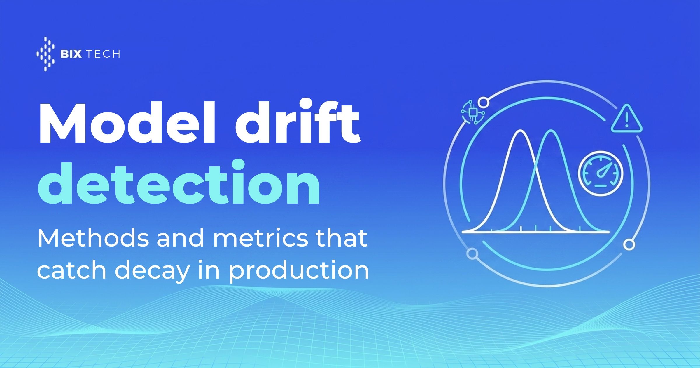
Model drift detection is what decides whether a model still deserves the traffic it receives. Offline validation says a model was good on a snapshot of the past. Production says nothing at all, unless someone measures it. Gartner expects organizations to abandon 60% of AI projects through 2026 for lack of AI-ready data and integration infrastructure, and a large share of that waste happens after go-live, when the world moves and the model quietly keeps answering as if nothing changed. Closing that gap is operational work, and it sits at the intersection of data science and platform engineering.
Regulation raised the stakes this year. Since August 2, 2026, the high-risk obligations of the EU AI Act apply in full, and Article 72 requires providers to run a documented post-market monitoring system that systematically collects and analyses performance data across the system's lifetime. Drift measurement stopped being a nice-to-have dashboard and became evidence, in the same way that audit trails became evidence for teams working on LLM governance.
What follows is a practical map: the four things people call drift, the methods and metrics that detect each one, how to set thresholds and windows without drowning the team in alerts, and what to do when a monitor fires. Every tool named here is one option among several, and the right combination depends on volume, label delay and the cost of a wrong prediction, the same situational logic that guides production RAG decisions.
Four things people call drift
The word "drift" gets stretched to cover any degradation, which makes incident calls confusing. Each signal has a different detection method, a different latency, and a different fix. Treating a shift in input data as if it were a shift in the input-to-outcome relationship leads to retraining a model that never had a modeling problem, only a broken upstream pipeline feeding it, which is why lineage and traceability belong next to monitoring.
| Signal | What shifted | How it is detected | Detection latency |
|---|---|---|---|
| Data drift (covariate shift) | The distribution of input features | Feature-by-feature comparison against a reference window | Immediate |
| Prediction drift | The distribution of model outputs | Output distribution compared with validation or recent production data | Immediate |
| Concept drift | The relationship between inputs and the target | Error monitoring over time, streaming change detectors | Waits for labels |
| Label drift | The distribution of the target itself | Ground truth compared with the training target distribution | Waits for labels |
| Data quality decay | Nulls, types, ranges, freshness, schema | Rule and constraint checks on the input contract | Immediate |
Prediction drift is the cheapest early warning, because model outputs exist the instant a request is served. When the output histogram moves, the diagnostic order is to find which input features moved first. Concept drift is the expensive one, since it only shows up once outcomes come back, and by then the model has been wrong for a while. That asymmetry is why teams pair a fast proxy signal with a slower ground-truth check, the same layering used when a semantic layer validates numbers before an agent consumes them.
Data quality decay deserves its own row because it masquerades as drift. A currency field arriving as a string, a sensor reporting zeros during maintenance, a join that silently duplicates rows: each produces a distribution change that no retraining fixes. Checking the input contract first saves entire afternoons, which argues for treating monitoring as part of the data engineering surface rather than a data science side project.
Methods and metrics for model drift detection
Every method answers one question: are these two samples, reference and current, drawn from the same distribution? The families differ in what they return. Statistical tests return a p-value, a yes-or-no verdict at a confidence level, while distance and divergence metrics return a magnitude you can trend over weeks. Choosing between them is mostly a question of sample size, and that choice shapes how noisy the monitor feels day to day for whoever runs the data platform.
Tests for small windows, distances for large ones
The default logic in Evidently's drift detection makes the tradeoff explicit. With 1,000 observations or fewer, it applies a two-sample Kolmogorov-Smirnov test to numerical columns, a chi-squared test to categorical columns, and a proportion difference test to binary features, flagging drift at a 0.95 confidence level, so a p-value at or below 0.05 means drift. Above 1,000 observations, it switches to Wasserstein distance for numerical columns and Jensen-Shannon divergence for categorical ones, with a default threshold of 0.1.
That switch is more than cosmetic. Hypothesis tests grow more sensitive as samples grow, so on a million daily requests a Kolmogorov-Smirnov test will report drift for a difference no human would care about. Distance metrics keep their meaning at any volume and give you a curve to watch, which fits high-traffic endpoints running behind containerized inference.
| Method | Applies to | What it returns | Common convention |
|---|---|---|---|
| Two-sample Kolmogorov-Smirnov | Numerical, continuous | p-value from the maximum CDF distance | Drift at p ≤ 0.05, small windows only |
| Pearson chi-squared | Categorical, low cardinality | p-value from expected vs observed counts | Drift at p ≤ 0.05, small windows only |
| Population Stability Index | Numerical (binned) and categorical | Bounded divergence score | Below 0.1 stable, 0.1 to 0.25 watch, above 0.25 act |
| Jensen-Shannon divergence | Categorical and numerical | Symmetric, bounded distance | Drift at 0.1 by default, tuned per feature |
| Wasserstein distance | Numerical, continuous | Cost of moving one distribution onto the other | Normalize by standard deviation, then threshold |
| Chebyshev distance | Prediction distributions | Maximum single-bin difference | Useful when one class share spikes |
Population Stability Index carries the most institutional history of the group. Credit risk teams have used the 0.1 and 0.25 bands for decades to decide whether a scorecard population still matches the one it was built on, which is why PSI keeps showing up in governance documents a regulator or an auditor will read. Managed monitors offer the same menu: Azure Machine Learning model monitoring supports Jensen-Shannon distance, PSI, normalized Wasserstein distance, the two-sample Kolmogorov-Smirnov test and Pearson's chi-squared test for data drift, adds Chebyshev distance for prediction drift, and tracks null value rate, data type error rate and out-of-bounds rate as separate data quality metrics. Amazon SageMaker Model Monitor covers a similar contract and is now closed to new customers, a reminder to keep the monitoring definition portable across whichever cloud platform the team standardizes on.
When one feature at a time is not enough
Per-feature tests miss correlation breaks. Two features can each keep a perfect marginal distribution while the relationship between them inverts, and the model that learned that relationship degrades anyway. Three approaches cover the gap: a domain classifier trained to tell reference rows from current rows, using its discriminative power as the drift score, which Evidently applies to text drift at a threshold of ROC AUC above 0.55; reconstruction error from a PCA or autoencoder fit on training data; and feature attribution drift, comparing feature importance rankings in production against training through normalized discounted cumulative gain. Each complements the per-feature view that most monitoring stacks ship by default.
Generative systems need the same idea applied to embeddings. In a retrieval pipeline, the useful monitors are the distribution of query embeddings, the similarity scores of retrieved chunks, and the share of retrievals below a relevance floor, since a corpus that grows in one topic and stagnates in another shifts retrieval quality long before anyone complains. Those signals fit into the span attributes that OpenTelemetry instrumentation already collects per request.
Streaming detectors for concept drift
When labels arrive quickly, concept drift is best detected on the error stream rather than on the inputs. The river library implements the classics from the streaming literature: ADWIN keeps an adaptive window over a running statistic and shrinks it when the recent regime stops matching the older one, DDM watches the error rate and its standard deviation and declares the predictor outdated when errors rise past a warning level, and Page-Hinkley tracks the cumulative deviation of an observation from the running mean. All three return a change point rather than a batch verdict, which suits fraud, pricing and recommendation models where the environment moves in hours instead of quarters, and where durable orchestration reacts without a human in the loop.
Monitoring when labels arrive late
Most business models learn whether they were right long after the prediction. A churn score gets confirmed in 90 days, a credit decision in 12 months, a maintenance alert whenever the part fails. Waiting for ground truth means accepting a quarter of blind operation, which is why label delay belongs in the same conversation as pipeline reliability.
Performance estimation fills the gap. NannyML's performance estimation documents two approaches: confidence-based performance estimation, which uses the calibrated class probabilities a classifier already returns to estimate a metric such as ROC AUC on unlabeled data, and direct loss estimation, which trains a second model to predict the loss of the monitored model per observation. Both assume the absence of concept drift, so they answer how the model behaves under a new input distribution rather than whether the target relationship changed. That boundary keeps the estimate honest when it feeds a retraining decision in a lakehouse or mesh setup.
Cheaper proxies help too, and most teams run several at once. Prediction distribution shifts, confidence collapse toward the decision boundary, segment-level volume changes and human override rates all correlate with quality loss and cost nothing extra to compute. A small labeled sample each week gives the monitoring layer a slow but real anchor, the discipline that keeps BI reporting trustworthy while automated checks do the heavy lifting.
Thresholds, windows and the runbook after an alert
A drift monitor is a comparison, so its credibility comes from the windows on both sides. Azure's guidance works as a template: training data as the reference for data drift and data quality, validation data as the reference for prediction drift, and no overlap between the two windows, since the default reference offset is twice the production window size precisely to guarantee enough independent data. Frequency follows traffic volume, daily for a busy endpoint and weekly or monthly when data accumulates slowly, and the same cost discipline that governs query spend applies to how often these jobs run.
Alert fatigue kills monitoring faster than bad math. Scoping drift checks to the top N features by importance keeps noise down on wide models, seasonal features deserve wider thresholds or year-over-year references, and a single feature crossing 0.1 rarely justifies paging anyone. A composite rule works better: escalate when a high-importance feature drifts and prediction drift moves in the same window, or when estimated performance drops below the service level the business agreed to, a logic close to what mature teams apply to agentic systems in production.
| Alert pattern | Most likely cause | First action |
|---|---|---|
| Data quality metrics move, distributions follow | Upstream pipeline or schema change | Fix the source, hold any retraining |
| One low-importance feature drifts | Real but harmless population change | Log it, widen the threshold, no action |
| High-importance features drift, quality holds | Population shift the model still handles | Watch weekly, prepare a training refresh |
| Prediction drift with stable inputs | Serving skew, wrong feature version, bad deploy | Compare feature values in training and serving, roll back if needed |
| Estimated or measured performance falls | Concept drift, the target relationship changed | Retrain on recent data, revalidate, consider new features |
| Everything drifts at once, sharply | Instrumentation or logging change | Verify the collection layer before touching the model |
Retraining is the action people reach for first and should reach for last, after the input contract has been cleared and the drift tied to something the model depends on. Automating the trigger works well when the pipeline is cheap and labels are fresh, and badly when each run costs a GPU day and ground truth is three months out. A practical middle ground automates detection and the candidate training run, then keeps a named human approval on promotion, with the metrics and model registry recording who approved what and against which evaluation.
Model drift detection earns its keep when the numbers connect to decisions: a metric per drift type, a threshold someone agreed to, a window that makes statistical sense, and a runbook that says what happens when the monitor fires. BIX Tech works across multiple cloud, data and machine learning platforms, and the right assembly of tests, distances and performance estimators depends on traffic volume, label delay and how much a silent wrong prediction costs the operation.
Detection is one layer of a larger system; how drift signals connect to deployment patterns and retraining across the platform is mapped in our MLOps reference architecture for 2026.
If your company runs models in production and needs model drift detection wired to real thresholds and clear actions, our specialists can help you design the monitoring layer for your context. Talk to our team and move forward with your data maturity. ⬇️

FAQ: model drift detection
What is model drift detection?
Model drift detection is the practice of measuring whether a production model's inputs, outputs or accuracy have moved away from the data it was trained and validated on. It compares a current production window against a reference window using statistical tests or distance metrics, then triggers an alert, an investigation or a retraining run when the difference crosses an agreed threshold.
What is the difference between data drift and concept drift?
Data drift is a change in the distribution of input features, detectable immediately from the request stream. Concept drift is a change in the relationship between those inputs and the target, so the same input should now produce a different outcome. Data drift can happen without hurting accuracy, while concept drift always degrades it and only becomes visible once labels arrive.
Which metrics are used to detect model drift?
The common set includes the two-sample Kolmogorov-Smirnov test and Pearson's chi-squared test for small windows, plus Population Stability Index, Jensen-Shannon divergence, Wasserstein distance and Chebyshev distance for larger ones. Azure Machine Learning model monitoring exposes exactly this menu, and Evidently defaults to hypothesis tests at or below 1,000 observations and to distance metrics above that.
What is a good PSI threshold for drift?
The convention inherited from credit scoring reads Population Stability Index below 0.1 as a stable population, 0.1 to 0.25 as moderate change worth watching, and above 0.25 as a shift significant enough to act on. Those bands are a starting point rather than a rule, and seasonal or low-importance features usually deserve wider bounds to avoid alert fatigue.
How do you monitor a model when labels arrive months later?
Combine proxy signals with performance estimation. Prediction drift, confidence collapse, segment volume changes and human override rates are available immediately, while methods such as confidence-based performance estimation and direct loss estimation approximate accuracy on unlabeled data. Both assume input drift rather than concept drift, so pair them with a small labeled sample as a slow ground-truth anchor.